Data Loading and Initial Data Analysis - Network Security Cookbook

Overview¶

This notebook introduces the curriculum. The focus is on understanding the initial state of the network traffic data (TII-SSRC-23 dataset) and assessing data quality before making any alterations. We perform an extensive exploratory data analysis (EDA) to understand the dataset’s structure, class balance, feature types, missing values, duplicates, impossible values, sparsity, and distributions. The findings here will serve as the blueprint for the active data cleaning steps in Notebook 2.

Learning Objectives¶

After working through this notebook, you will be able to:

Assess dataset dimensionality and target class balance.
Distinguish numerical features from categorical ones (even when they are stored as integers).
Compute extended summary statistics (including zero and negative counts).
Detect missing values, exact duplicates, and imposisble values (e.g. negative time, invalid ports).
Quantify sparsity (percentage of zeros) and interpret its impact on high-dimensional data.
Visualise heavy-tailed distributions using objective binning rules (Doane, Freedman-Diaconis) and Q-Q plots.

Prerequisites¶

A basic understanding of Python, Pandas data structures, and statistical concepts (mean, min, max, distributions, skewness).
Ensure that the required libraries pandas, numpy, matplotlib, seaborn and statsmodels are installed. If you are running this notebook in a Binder environment, the necessary dependencies should already be installed.
Access to the TII-SSRC-23 dataset, which is available in the GitLab data repository. Alternatively, you can run this notebook locally and download the dataset from Kaggle. If you run this notebook in Binder, the dataset is already provided within the environment.

Content / Key Steps¶

References & Acknowledgements¶

Primary Dataset: article{herzalla2023tii, title={TII-SSRC-23 Dataset: Typological Exploration of Diverse Traffic Patterns for Intrusion Detection}, author={Herzalla, Dania and Lunardi, Willian T and Andreoni, Martin}, journal={IEEE Access}, year={2023}, publisher={IEEE}, doi={10.1109/ACCESS.2023.3319213} }
Methodological Context: R. Flood, G. Engelen, D. Aspinall and L. Desmet, “Bad Design Smells in Benchmark NIDS Datasets,” 2024 IEEE 9th European Symposium on Security and Privacy (EuroS&P), Vienna, Austria, 2024, pp. 658-675, doi: 10.1109/EuroSP60621.2024.00042.
Contributions: Francesca Ricter; Konstantinos Vakalopoulos

1. Imports¶

We import standard data science libraries and several custom utility functions for plotting.

import pandas as pd

from network_security_cookbook.utils import (
    plot_distributions,
    plot_q_qplots,
    print_package_versions,
)

Now we will print the versions of the key libraries we are using.

print_package_versions()

matplotlib: 3.10.9
numpy: 2.4.6
pandas: 3.0.3
seaborn: 0.13.2
statsmodels: 0.14.6

2. Load the Dataset¶

First, we will load the CSV dataset directly from a URL into a Pandas DataFrame. The dataset is available as a CSV file hosted on TU GitLab. If access to the repository containing the dataset is restricted, you can download it from Kaggle and load it from a local path instead. The link to the dataset in Kaggle is provided in the introduction section of this notebook.

TU GitLab¶

DATASET_URL = "https://gitlab.tuwien.ac.at/api/v4/projects/11927/repository/files/sampled_data.csv/raw?ref=main&lfs=true"

BinderHub¶

(Uncomment if running in Binder)

# DATASET_URL = "/home/jovyan/cookbooks-input-data/network-security-cookbook/tii-ssrc-23.csv"

Loading¶

Here we actually load the dataset. Make sure to adjust the DATASET_URL variable to point to the correct location of the dataset.

%%time
df = pd.read_csv(DATASET_URL)

CPU times: user 4.2 s, sys: 28.1 s, total: 32.3 s
Wall time: 33 s

3. Initial Data Exploration¶

We systematically examine the dataset to understand its overall structure, characteristics, and immediately identify potential problems.

3.1. Dataset Overview and Class Balance¶

First, we check the shape and the distribution of the target labels.

Number of samples and features¶

We use the .shape property to check the dimensionality.

n_samples, n_features_total = df.shape

print(f"Number of samples (rows): {n_samples}")
print(f"Number of features (columns): {n_features_total}")
print("\nColumn names:", list(df.columns))

Number of samples (rows): 432831
Number of features (columns): 86

Column names: ['Flow ID', 'Src IP', 'Src Port', 'Dst IP', 'Dst Port', 'Protocol', 'Timestamp', 'Flow Duration', 'Total Fwd Packet', 'Total Bwd packets', 'Total Length of Fwd Packet', 'Total Length of Bwd Packet', 'Fwd Packet Length Max', 'Fwd Packet Length Min', 'Fwd Packet Length Mean', 'Fwd Packet Length Std', 'Bwd Packet Length Max', 'Bwd Packet Length Min', 'Bwd Packet Length Mean', 'Bwd Packet Length Std', 'Flow Bytes/s', 'Flow Packets/s', 'Flow IAT Mean', 'Flow IAT Std', 'Flow IAT Max', 'Flow IAT Min', 'Fwd IAT Total', 'Fwd IAT Mean', 'Fwd IAT Std', 'Fwd IAT Max', 'Fwd IAT Min', 'Bwd IAT Total', 'Bwd IAT Mean', 'Bwd IAT Std', 'Bwd IAT Max', 'Bwd IAT Min', 'Fwd PSH Flags', 'Bwd PSH Flags', 'Fwd URG Flags', 'Bwd URG Flags', 'Fwd Header Length', 'Bwd Header Length', 'Fwd Packets/s', 'Bwd Packets/s', 'Packet Length Min', 'Packet Length Max', 'Packet Length Mean', 'Packet Length Std', 'Packet Length Variance', 'FIN Flag Count', 'SYN Flag Count', 'RST Flag Count', 'PSH Flag Count', 'ACK Flag Count', 'URG Flag Count', 'CWR Flag Count', 'ECE Flag Count', 'Down/Up Ratio', 'Average Packet Size', 'Fwd Segment Size Avg', 'Bwd Segment Size Avg', 'Fwd Bytes/Bulk Avg', 'Fwd Packet/Bulk Avg', 'Fwd Bulk Rate Avg', 'Bwd Bytes/Bulk Avg', 'Bwd Packet/Bulk Avg', 'Bwd Bulk Rate Avg', 'Subflow Fwd Packets', 'Subflow Fwd Bytes', 'Subflow Bwd Packets', 'Subflow Bwd Bytes', 'FWD Init Win Bytes', 'Bwd Init Win Bytes', 'Fwd Act Data Pkts', 'Fwd Seg Size Min', 'Active Mean', 'Active Std', 'Active Max', 'Active Min', 'Idle Mean', 'Idle Std', 'Idle Max', 'Idle Min', 'Label', 'Traffic Type', 'Traffic Subtype']

Distribution of Labels¶

Next, we will examine the distribution of our target labels. This is a critical step to check for class imbalance, which can significantly impact the performance of machine learning models.

# Class balance for binary classification
label_counts = df["Label"].value_counts()
label_percent = df["Label"].value_counts(normalize=True) * 100

balance_df = pd.DataFrame({"Instances": label_counts, "Percentage (%)": label_percent})

print("Class distribution (Label):")
print(balance_df)

Class distribution (Label):

           Instances  Percentage (%)
Label                               
Malicious     432757       99.982903
Benign            74        0.017097

# Also check Traffic Type and Subtype
print("Traffic Type distribution:")
print(df["Traffic Type"].value_counts())

print("\nTraffic Subtype distribution:")
print(df["Traffic Subtype"].value_counts())

Traffic Type distribution:

Traffic Type
DoS                      374563
Information Gathering     51863
Mirai                      4553
Bruteforce                 1778
Video                        49
Audio                        12
Text                         12
Background                    1
Name: count, dtype: int64

Traffic Subtype distribution:
Traffic Subtype
DoS RST                  53739
Information Gathering    51863
DoS ACK                  46799
DoS PSH                  45460
DoS URG                  45291
DoS CWR                  43720
DoS ECN                  43435
DoS SYN                  42882
DoS FIN                  36310
DoS UDP                  12831
DoS HTTP                  4094
Mirai DDoS DNS            2785
Bruteforce DNS            1145
Mirai DDoS SYN             714
Mirai DDoS HTTP            449
Mirai Scan Bruteforce      428
Bruteforce Telnet          235
Bruteforce SSH             212
Mirai DDoS ACK             172
Bruteforce FTP             158
Bruteforce HTTP             28
Video HTTP                  27
Video RTP                   14
Audio                       12
Text                        12
Video UDP                    8
Mirai DDoS UDP               4
DoS MAC                      2
Background                   1
Mirai DDoS GREIP             1
Name: count, dtype: int64

3.2. Feature Types: Numerical vs. Categorical¶

Machine learning algorithms perform mathematical operations, which means they cannot natively process raw text or categorical data. Therefore, we must distinguish between numerical and categorical features.

Numerical Features: Represent quantities and magnitudes (e.g. Packet Length, Flow Duration).
Categorical Features: Represent qualitative data or nominal identifiers (e.g. Src IP, Protocol).

Pandas automatically infers data types, but this inference is often flawed in network datasets. For example, Src Port and Dst Port are represented as numbers, but they are actually categorical identifiers.

df_numerical = df.select_dtypes(include=["number"])
print(f"Columns automatically detected as numeric: {len(df_numerical.columns)}")
print(list(df_numerical.columns))

Columns automatically detected as numeric: 79
['Src Port', 'Dst Port', 'Protocol', 'Flow Duration', 'Total Fwd Packet', 'Total Bwd packets', 'Total Length of Fwd Packet', 'Total Length of Bwd Packet', 'Fwd Packet Length Max', 'Fwd Packet Length Min', 'Fwd Packet Length Mean', 'Fwd Packet Length Std', 'Bwd Packet Length Max', 'Bwd Packet Length Min', 'Bwd Packet Length Mean', 'Bwd Packet Length Std', 'Flow Bytes/s', 'Flow Packets/s', 'Flow IAT Mean', 'Flow IAT Std', 'Flow IAT Max', 'Flow IAT Min', 'Fwd IAT Total', 'Fwd IAT Mean', 'Fwd IAT Std', 'Fwd IAT Max', 'Fwd IAT Min', 'Bwd IAT Total', 'Bwd IAT Mean', 'Bwd IAT Std', 'Bwd IAT Max', 'Bwd IAT Min', 'Fwd PSH Flags', 'Bwd PSH Flags', 'Fwd URG Flags', 'Bwd URG Flags', 'Fwd Header Length', 'Bwd Header Length', 'Fwd Packets/s', 'Bwd Packets/s', 'Packet Length Min', 'Packet Length Max', 'Packet Length Mean', 'Packet Length Std', 'Packet Length Variance', 'FIN Flag Count', 'SYN Flag Count', 'RST Flag Count', 'PSH Flag Count', 'ACK Flag Count', 'URG Flag Count', 'CWR Flag Count', 'ECE Flag Count', 'Down/Up Ratio', 'Average Packet Size', 'Fwd Segment Size Avg', 'Bwd Segment Size Avg', 'Fwd Bytes/Bulk Avg', 'Fwd Packet/Bulk Avg', 'Fwd Bulk Rate Avg', 'Bwd Bytes/Bulk Avg', 'Bwd Packet/Bulk Avg', 'Bwd Bulk Rate Avg', 'Subflow Fwd Packets', 'Subflow Fwd Bytes', 'Subflow Bwd Packets', 'Subflow Bwd Bytes', 'FWD Init Win Bytes', 'Bwd Init Win Bytes', 'Fwd Act Data Pkts', 'Fwd Seg Size Min', 'Active Mean', 'Active Std', 'Active Max', 'Active Min', 'Idle Mean', 'Idle Std', 'Idle Max', 'Idle Min']

df_categorical = df.select_dtypes(exclude=["number"])
print(f"Columns automatically detected as category: {len(df_categorical.columns)}")
print(list(df_categorical.columns))

Columns automatically detected as category: 7
['Flow ID', 'Src IP', 'Dst IP', 'Timestamp', 'Label', 'Traffic Type', 'Traffic Subtype']

3.3. Extended Summary Statistics for Numerical Features (Feature Statistics)¶

Next, we generate summary statistics for our features. We enhanced the standard .describe() by adding zero count, negative count and missing count for each numerical column.

# Manually identified categorical columns stored as integers
categorical_as_int = ["Src Port", "Dst Port", "Protocol"]

# Use only true numerical features (exclude the categorical-as-int columns for now)
true_numeric_cols = [
    col for col in df_numerical.columns if col not in categorical_as_int
]
df_true_numeric = df_numerical[true_numeric_cols]

# Compute extended stats
desc = df_true_numeric.describe().T  # transpose for easier adding
desc["zero_count"] = (df_true_numeric == 0).sum()
desc["zero_percent"] = (df_true_numeric == 0).mean() * 100
desc["negative_count"] = (df_true_numeric < 0).sum()
desc["missing_count"] = df_true_numeric.isna().sum()

# Reorder columns for readability
desc = desc[
    [
        "count",
        "missing_count",
        "zero_count",
        "zero_percent",
        "negative_count",
        "mean",
        "std",
        "min",
        "25%",
        "50%",
        "75%",
        "max",
    ]
]
print("Extended summary statistics (first 15 features):")
desc.head(15)

Extended summary statistics (first 15 features):

Loading...

4. Data Quality and Sanity Checks¶

In this section, we actively look for general data quality issues that will need to be cleaned.

4.1. Duplicate Rows¶

Duplicate samples can severely bias machine learning models by artificially inflating the importance of certain patterns and causing “data leakage” (where identical samples end up in both the training and testing sets).

duplicate_count = df.duplicated().sum()
print(f"Number of exact duplicate rows: {duplicate_count}")

if duplicate_count > 0:
    dup_samples = df[df.duplicated(keep=False)]
    print("\nClass distribution among duplicates:")
    print(dup_samples["Label"].value_counts())
    print("\nTraffic Type distribution among duplicates:")
    print(dup_samples["Traffic Type"].value_counts())

Number of exact duplicate rows: 0

4.2. Missing Values¶

Although the summary above shows zero missing values (NaN or null values) in numeric columns, we double-check the entire DataFrame. Most machine learning algorithms cannot handle missing data out-of-the-box.

missing_total = df.isna().sum().sum()
print(f"Total missing values in entire dataset: {missing_total}")

if missing_total == 0:
    print("No missing values – dataset is complete.")
else:
    print("Columns with missing values:")
    print(df.isna().sum()[df.isna().sum() > 0])

Total missing values in entire dataset: 0
No missing values – dataset is complete.

# Per-class missingness
missing_per_class = (
    df.groupby("Label").apply(lambda x: x.isna().sum().sum()).rename("Missing_Entries")
)
missing_pct = (missing_per_class / (n_samples * df.shape[1]) * 100).round(4)
missing_table = pd.DataFrame(
    {"Missing_Entries": missing_per_class, "Missing_%_of_Total_Cells": missing_pct}
)
print("Missingness by Class")
display(missing_table)

Missingness by Class

Loading...

4.3. Sanity Checks: Impossible Values¶

We look for values that are logically impossible in network traffic. Features like time duration, packet length, and byte counts cannot logically be negative. Furthermore, certain categorical values might be invalid (e.g. a port number of -1).

Negative values (time, length, counts)¶

Features like Flow IAT Min, Fwd IAT Min, Bwd IAT Min represent inter-arrival time intervals, they cannot be negative.

neg_cols = (df_true_numeric < 0).any()
neg_cols = neg_cols[neg_cols == True].index.tolist()
print(f"Columns containing negative values: {neg_cols}")

if neg_cols:
    # How many samples have negative values and what are their labels?
    for col in neg_cols:
        neg_count = (df_true_numeric[col] < 0).sum()
        print(f"  {col}: {neg_count} negative values")
else:
    print("No negative values found.")

Columns containing negative values: ['Flow IAT Min']
  Flow IAT Min: 2 negative values

Invalid port numbers¶

Port numbers must be in $[0,65535]$ . -1 usually indicates parsing errors.

for port_col in ["Src Port", "Dst Port"]:
    invalid = df[~df[port_col].between(0, 65535)]
    print(f"{port_col}: {len(invalid)} invalid entries")

    if len(invalid) > 0:
        print(invalid[[port_col, "Label"]].head())

Src Port: 0 invalid entries
Dst Port: 0 invalid entries

Invalid protocol numbers¶

Typical IP protocol numbers range from 0 to 255 (e.g. TCP=6, UDP=17).

invalid_proto = df[~df["Protocol"].between(0, 255)]
print(f"Invalid protocol numbers: {len(invalid_proto)}")
if len(invalid_proto) > 0:
    print(invalid_proto["Protocol"].unique())

Invalid protocol numbers: 0

4.4. Sparsity and Zero Values¶

Network traffic data is notoriously sparse (contains many zeros). Many features (like specific TCP flags or backward bulk rates) are inactive for the vast majority of connections. We will calculate the percentage of zero values for each numerical feature.

Earlier we looked at the zero percentages per column (feature). Now, let’s examine the absolute counts. We use sum().sum() to get the total number of zero entries across the entire matrix.

print(
    f"Total zero entries across all numerical features: {(df_numerical == 0).sum().sum()}"
)

Total zero entries across all numerical features: 19910569

Now we look at the percentages for the features with zeros.

zero_percent = (df_true_numeric == 0).mean() * 100
high_sparsity = zero_percent[zero_percent > 80].sort_values(ascending=False)

print(f"Features with more than 80% zeros: {len(high_sparsity)}")
print(high_sparsity)

Features with more than 80% zeros: 37
Fwd Bulk Rate Avg             100.000000
Fwd Packet/Bulk Avg           100.000000
Fwd Bytes/Bulk Avg            100.000000
Bwd PSH Flags                 100.000000
Bwd URG Flags                 100.000000
Bwd Bulk Rate Avg              99.828108
Bwd Bytes/Bulk Avg             99.828108
Bwd Packet/Bulk Avg            99.828108
Bwd Packet Length Min          99.699421
Bwd IAT Std                    99.394683
Subflow Bwd Bytes              99.387752
Bwd Packet Length Std          99.367421
Bwd IAT Min                    99.337155
Bwd IAT Max                    99.316823
Bwd IAT Mean                   99.316823
Bwd IAT Total                  99.316823
Bwd Init Win Bytes             99.213319
Bwd Segment Size Avg           99.117901
Bwd Packet Length Mean         99.117901
Bwd Packet Length Max          99.117901
Total Length of Bwd Packet     99.117901
Active Std                     98.481393
Active Max                     90.347734
Active Min                     90.347734
Active Mean                    90.347734
ECE Flag Count                 89.965137
CWR Flag Count                 89.899060
Idle Std                       88.495741
FIN Flag Count                 88.487886
Fwd URG Flags                  88.124926
URG Flag Count                 88.119844
Fwd PSH Flags                  87.542944
SYN Flag Count                 86.970896
PSH Flag Count                 86.794615
Subflow Bwd Packets            85.472390
Fwd Packet Length Std          84.682474
Fwd IAT Std                    81.968944
dtype: float64

4.5. Summary of Data Quality Issues¶

Let’s summarize our findings in two comprehensive tables.

Table 1: Sample-Level Quality Summary¶

This table shows the absolute count and percentage of samples (rows) affected by various issues.

total_samples = len(df)
num_missing_samples = df.isnull().any(axis=1).sum()
num_duplicate_samples = df.duplicated(keep=False).sum()
num_negative_samples = (df_numerical < 0).any(axis=1).sum()

sample_summary = pd.DataFrame(
    {
        "Issue": [
            "Missing Values (NaN)",
            "Exact Duplicates",
            "Unplausible (Negative) Values",
        ],
        "Affected Samples": [
            num_missing_samples,
            num_duplicate_samples,
            num_negative_samples,
        ],
        "Percentage of Total (%)": [
            (num_missing_samples / total_samples) * 100,
            (num_duplicate_samples / total_samples) * 100,
            (num_negative_samples / total_samples) * 100,
        ],
    }
)

print("Sample-Level Data Quality Summary:")
print(sample_summary.to_string(index=False))

Sample-Level Data Quality Summary:
                        Issue  Affected Samples  Percentage of Total (%)
         Missing Values (NaN)                 0                 0.000000
             Exact Duplicates                 0                 0.000000
Unplausible (Negative) Values                 2                 0.000462

Table 2: Feature-Level Quality Summary¶

Highlights features suffering from extreme sparsity or zero variance. We will filter out the features that have 0 issues to focus on the problematic ones.

feature_summary = pd.DataFrame(index=df_numerical.columns)
feature_summary["% Missing"] = df_numerical.isnull().mean() * 100
feature_summary["% Negative"] = (df_numerical < 0).mean() * 100
feature_summary["% Zeros"] = (df_numerical == 0).mean() * 100

# Also let's highlight "Zero Variance" features (features where all values are identical, e.g. 100% zeros)
feature_summary["Is Zero Variance"] = df_numerical.nunique() <= 1

# Display top 15 features with highest percentage of zeros
print("Feature-Level Quality Summary (Top 15 sparse features):")
print(feature_summary.sort_values(by="% Zeros", ascending=False).head(15).round(4))

Feature-Level Quality Summary (Top 15 sparse features):
                       % Missing  % Negative   % Zeros  Is Zero Variance
Fwd Bulk Rate Avg            0.0         0.0  100.0000              True
Bwd PSH Flags                0.0         0.0  100.0000              True
Fwd Packet/Bulk Avg          0.0         0.0  100.0000              True
Fwd Bytes/Bulk Avg           0.0         0.0  100.0000              True
Bwd URG Flags                0.0         0.0  100.0000              True
Bwd Bytes/Bulk Avg           0.0         0.0   99.8281             False
Bwd Packet/Bulk Avg          0.0         0.0   99.8281             False
Bwd Bulk Rate Avg            0.0         0.0   99.8281             False
Bwd Packet Length Min        0.0         0.0   99.6994             False
Bwd IAT Std                  0.0         0.0   99.3947             False
Subflow Bwd Bytes            0.0         0.0   99.3878             False
Bwd Packet Length Std        0.0         0.0   99.3674             False
Bwd IAT Min                  0.0         0.0   99.3372             False
Bwd IAT Mean                 0.0         0.0   99.3168             False
Bwd IAT Max                  0.0         0.0   99.3168             False

5. Data Distribution Analysis & Normality Assessment¶

To truly understand the skewness of our data, we need to plot histograms. However, the shape of a histogram is highly sensitive to the number of bins used. If we guess the bin count, important patterns may be hidden. Therefore, we use mathematical formulas tailored for non-normal, highly skewed data to objectively calculate optimal bin sizes.

Doane’s Rule is particularly useful when dealing with non-normal data as it accounts for skewness.
Freedman-Diaconis Rule uses the interquartile range and is very robust to outliers.

5.1. Doane’s Rule¶

Histograms using Doane’s rule.

plot_distributions(df_numerical, hist_bins="doane")

5.2. Freedman–Diaconis Rule¶

Histograms using Freedman-Diaconis rule.

plot_distributions(df_numerical, hist_bins="fd")

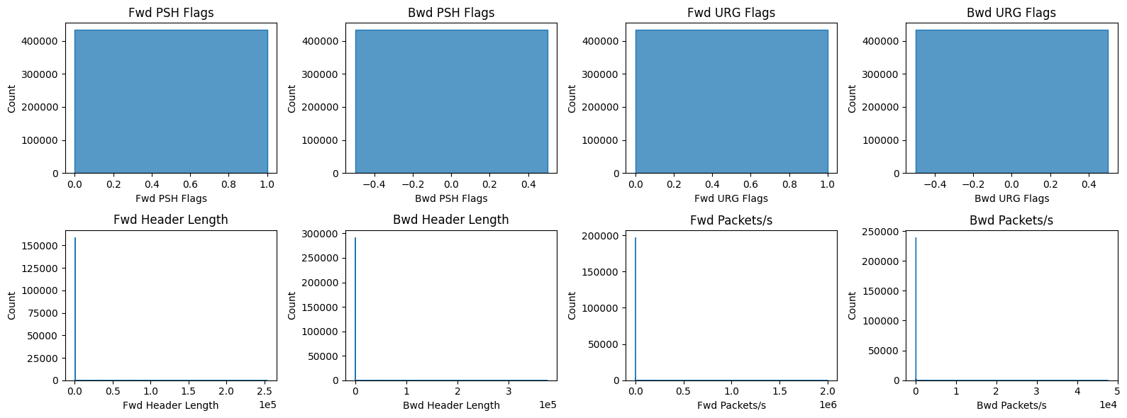
We want to plot a few heavily zero-inflated features separately.

plot_distributions(
    df_numerical[
        [
            "Bwd PSH Flags",
            "Bwd URG Flags",
            "Fwd Bytes/Bulk Avg",
            "Fwd Packet/Bulk Avg",
            "Fwd Bulk Rate Avg",
        ]
    ],
    hist_bins=4,
)

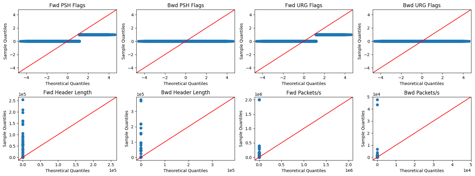
5.3. Q-Q Plots¶

A Quantile-Quantile (Q-Q) Plot compares our data’s distribution against a theoretical normal distribution. If the data is normally distributed, the points will form a straight 45-degree line.

plot_q_qplots(df_numerical)

6. Summary of Findings¶

Based on our EDA, the following issues must be addressed in the Data Cleaning pipeline (Notebook 2):

Issue	Example	Recommended action
Class imbalance	11% Benign, 89% Malicious	Resampling or class weights during modeling.
Categorical columns stored as int	`Src Port`, `Dst Port`, `Protocol`	Convert to `str` / isolate from numerical matrix / one‑hot encode.
Exact duplicate rows	1,802 duplicates	Drop duplicates to prevent data leakage.
Negative values	`Flow IAT Min` = -1	Drop corrupted rows (only 2).
Invalid port numbers	`Src Port` = -1	Drop rows (or set to 0).
Constant columns	Features with single unique value	Remove entirely (Zero Variance Filter).
Non‑behavioural identifiers	`Flow ID`, `Timestamp`	Remove to prevent model bias/leakage.
High sparsity	>80% zeros for many features	Consider dropping or map overlapping zero patterns for PCA.
Non‑normal distributions	Extreme skewness in Q-Q plots	Use non‑parametric correlation analysis (e.g. Spearman/Kendall).

7. Wrap-up & Checkpoint¶

We have successfully:

Profiled the dataset dimensions and class imbalance.
Distinguished logical (categorical) vs. physical (numerical) feature types.
Generated comprehensive feature-level statistics.
Identified duplicates, missingness, and physically impossible values.
Established a decision framework for data cleaning.
Confirmed heavy-tailed, non-normal distributions requiring non-parametric statistics.

Next Steps (Notebook 2):

Apply the decision framework to drop duplicates, zero-variance features, and invalid rows.
Cast categorical identifiers to strings to prevent false ordinal relationships.
Analyse and map overlapping zero patterns to prepare for dimensionality reduction.

📝 Summary Questions

Why is treating Port as a continuous number not good?
How does class imbalance affect the reliability of accuracy as a metric?
If a feature has 95% zeros, how does that affect Euclidean distance calculations?
When should you drop a feature vs. drop samples containing missing values?
Why did we reject Pearson correlation in favor of Spearman correlation?